用声音预测性别
实验目的
熟悉使用R语言进行大数据综合分析的方法
实验原理
R工具是一套完整的的数据处理计算和制图软件系统。其功能包括:数据存储和处理系统;数组运算工具(其向量、矩阵运算方面功能尤其强大);完整连贯的统计分析工具;优秀的的统计制图功能;简便而强大的的编程语言:可操纵数据的输入和输出以及可实现分支、循环等用户自定义功能。
实验背景
随着人工智能的算法发展,对于非结构化数据的处理能力越来越受到重视,这里面的关键一环就是语音数据的处理。目前,许多关于语音识别的应用案例已经影响着我们的生活,例如一些智能音箱中利用语音发送指令,一些搜索工具利用语音输出文本代替键盘录入。
未见其人,先闻其声。人类能够根据一段声音,大概率地正确判别这段声音所属者的性别。好奇的你有没有想过人类究竟是如何做到这一点的?这个数据集是根据声音和语言的声学特性来识别男性或女性的声音。数据集包括3168个录音样本,从男性和女性的扬声器中收集。语音样本是用声波和调谐器封装的声波分析在R中进行预处理的,分析频率范围为0hz -280hz。
本案例将从数据导入,清理整理一直到最后根据数据利用多个算法建模,交叉验证以及多个预测模型,全方位地揭开人类判别声音性别的奥秘。
实验步骤
- 熟悉R环境;
- 打开R云件环境;
- 在相应编程环境中修改和运行代码;
- 查看结果。
实验一:数据读取
从Kaggle下载数据集:下载 导入数据和必要的包,如提示包不存在可以用install.packages("包名")的方式安装
require('readr')
require('ggplot2')
require('dplyr')
require('tidyr')
require('caret')
require('corrplot')
require('Hmisc')
require('parallel')
require('doParallel')
require('ggthemes')
require('e1071')
### read in original dataset
voice_Original <- read.csv("voice.csv",header = TRUE)
实验二:数据探索
我们可以看出我们共有21个变量,共计3168个观测值。
- meanfreq: mean frequency (in kHz)
- sd: standard deviation of frequency
- median: median frequency (in kHz)
- Q25: first quantile (in kHz)
- Q75: third quantile (in kHz)
- IQR: interquantile range (in kHz)
- skew: skewness (see note in specprop description)
- kurt: kurtosis (see note in specprop description)
- sp.ent: spectral entropy
- sfm: spectral flatness
- mode: mode frequency
- centroid: frequency centroid (see specprop)
- peakf: peak frequency (frequency with highest energy)
- meanfun: average of fundamental frequency measured across acoustic signal
- minfun: minimum fundamental frequency measured across acoustic signal
- maxfun: maximum fundamental frequency measured across acoustic signal
- meandom: average of dominant frequency measured across acoustic signal
- mindom: minimum of dominant frequency measured across acoustic signal
- maxdom: maximum of dominant frequency measured across acoustic signal
- dfrange: range of dominant frequency measured across acoustic signal
- modindx: modulation index. Calculated as the accumulated absolute difference between adjacent measurements of fundamental frequencies divided by the frequency range
- label: male or female
实验三:数据预处理
由于本数据集数据完整,没有缺失值,因而我们实际上并没有缺失值的挑战,但是为了跟实际的数据挖掘过程相匹配,我们会人为将一些数据设置为缺失值,并对这些缺失值进行插补,大家也可以实际看一下我们应用的插补法的效果
###missing values
## set 30 numbers in the first column into NA
set.seed(1001)
random_Number <- sample(1:3168,30)
voice_Original1 <- voice_Original
voice_Original[random_Number,1] <- NA
describe(voice_Original)

meanfreq
      n missing  unique    Info    Mean     .05     .10     .25
   3138      30    3136       1  0.1808  0.1257  0.1411  0.1635
    .50     .75     .90     .95
 0.1848  0.1991  0.2176  0.2291

lowest : 0.03936 0.04825 0.05965 0.05978 0.06218
highest: 0.24353 0.24436 0.24704 0.24964 0.25112
……
这时候我们能看见,第一个变量meanfreq 中有了30个缺失值,现在我们需要对他们进行插补,我们会用到caret 包中的preProcess 函数:
### impute missing data
original_Impute <- preProcess(voice_Original,method="bagImpute")
voice_Original <- predict(original_Impute,voice_Original)
现在我们来看一下我们插补法的结果,我们的方法就是将我们设为缺失值的原始值和我们插补后的值结合到一个数据框中,大家可以进行直接比较:
### compare results of imputation
compare_Imputation <- data.frame(
  voice_Original1[random_Number,1],
  voice_Original[random_Number,1]
)
compare_Imputation
对比结果如下:
    meanfreq meanfreq.1
1  0.2122875  0.2117257
2  0.1826562  0.1814900
3  0.2009399  0.1954627
4  0.1838745  0.1814900
5  0.1906527  0.1954627
6  0.2319645  0.2313031
7  0.1736314  0.1814900
8  0.2243824  0.2313031
9  0.1957448  0.1954627
10 0.2159557  0.2117257
11 0.2047696  0.2084277
12 0.1831099  0.1814900
13 0.1873643  0.1814900
14 0.2077344  0.2117257
15 0.1648246  0.1651041
16 0.1885224  0.1898701
17 0.1342805  0.1272604
18 0.1933665  0.1954627
19 0.1888149  0.1940667
20 0.2180404  0.2117257
21 0.1980392  0.1954627
22 0.1898704  0.1954627
23 0.1761953  0.1814900
24 0.2356528  0.2313031
25 0.1785359  0.1814900
26 0.1856824  0.1814900
27 0.1808664  0.1814900
28 0.1784912  0.1814900
29 0.1990789  0.1954627
30 0.1714903  0.1651041
可以看出,我们的插补出来的值和原始值之间的差异是比较小的,可以帮助我们进行下一步的建模工作。
另外一点,我们在实际工作中,我们用到的预测因子中,往往包含数值型和类别型的数据,但是我们数据中全部都是数值型的,所以我们要增加难度,将其中的一个因子转换为类别型数据,具体操作如下:
### add a categorcial variable
voice_Original <- voice_Original%>%
  mutate(sp.ent=
           ifelse(sp.ent>0.9,"High","Low"))
实验四:分析建模
我们关注的是,预测因子之间是不是存在高度的相关性,因为预测因子间的相关性对于一些模型,是有不利的影响的。 对于研究预测因子间的相关性,corrplot 包中的corrplot函数提供了很直观的图形方法:
###find correlations between factors
voice_Original <- voice_Original%>%
  mutate(sp.ent=
           ifelse(sp.ent>0.9,"High","Low"))
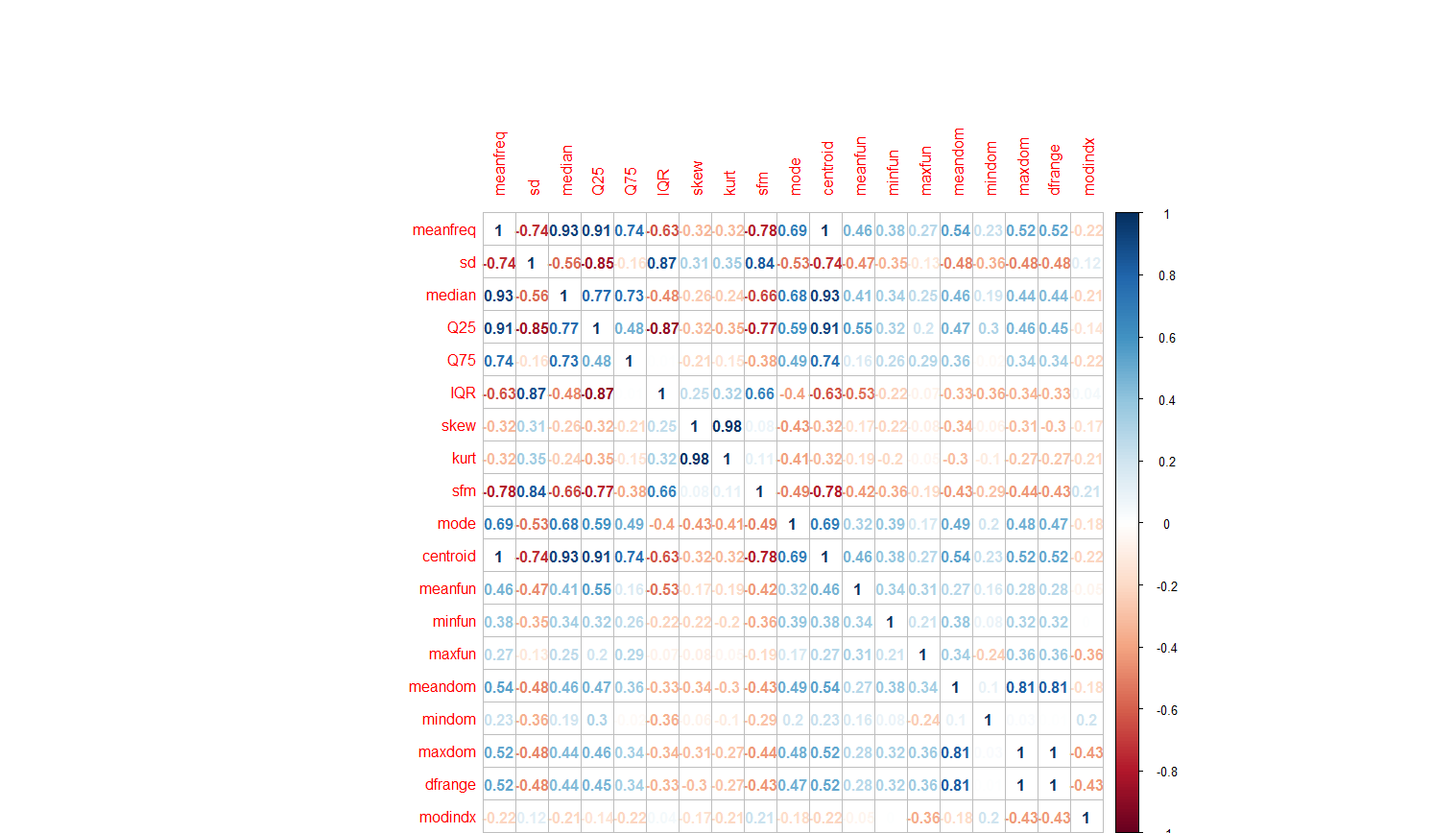
这个相关性矩阵图可以直观地帮助我们发现因子间的强相关性。
在实际建模过程中,我们不会将所有的数据全部用来进行训练模型,因为相比较模型数据集在训练中的表现,我们更关注模型在训练集,也就是我们的模型没有遇到的数据中的预测表现。
因此,我们将我们的数据集的70%的数据用来训练模型,剩余的30%用来检验模型预测的结果。
### separate dataset into training and testing sets
sample_Index <- createDataPartition(voice_Original$label,p=0.7,list=FALSE)
voice_Train <- voice_Original[sample_Index,]
voice_Test <- voice_Original[-sample_Index,]
但是我们还没有解决之前我们发现的一些问题,数据的量纲实际上是不一样的,另外某些因子间存在高度的相关性,这对我们的建模是不利的,因此我们需要进行一些预处理,我们又需要用到preProcess 函数:
### preprocess factors for further modeling
pp <- preProcess(voice_Train,method=c("scale","center","pca"))
voice_Train <- predict(pp,voice_Train)
voice_Test <- predict(pp,voice_Test)
现在,我们进行一些通用的设置,为不同的模型进行交叉验证比较做好准备。
### define formula
model_Formula <- label~PC1+PC2+PC3+PC4+PC5+PC6+PC7+PC8+PC9+PC10+sp.ent


###set cross-validation parameters

modelControl <- trainControl(method="repeatedcv",number=5,
                             repeats=5,allowParallel=TRUE)
下面我们开始建立我们的第一个模型:逻辑回归模型:
### model 1: logistic regression
glm_Model <- train(model_Formula,
                   data=voice_Train,
                   method="glm",
                   trControl=modelControl)
下面我们再来看看下一个模型:线性判别分析(LDA):
### model 2:linear discrimant analysis
lda_Model <- train(model_Formula,
                   data=voice_Train,
                   method="lda",
                   trControl=modelControl)
第三个模型:随机森林:
### model 3: random forrest
rf_Model <- train(model_Formula,
                  data=voice_Train,
                  method="rf",
                  trControl=modelControl,
                  ntrees=500)
实验五:模型评价与优化
将模型应用到测试集上,并将结果与真实值进行比较:
随机森林
voice_Test1 <- voice_Test[,-2]
voice_Test1$glmPrediction <- predict(glm_Model,voice_Test1)
table(voice_Test$label,voice_Test1$glmPrediction)

         female male
  female    459   16
  male        7  468
LDA
voice_Test1$ldaPrediction <- predict(lda_Model,voice_Test1)
table(voice_Test$label,voice_Test1$ldaPrediction)

         female male
  female    454   21
  male        6  469
随机森林
voice_Test1$rfPrediction <- predict(rf_Model,voice_Test1)
table(voice_Test$label,voice_Test1$rfPrediction)

       female male
  female    457   18
  male        6  469
可以看到随机森林的结果介于上面两个模型之间。但是模型的结果是存在一定的偶然性的,即因为都使用了交叉验证,每个模型都存在抽样的问题,因此结果之间存在一定的偶然性,所以我们需要对模型进行统计意义上的比较。
### which model is the best?
model_Comparison <-
  resamples(list(
    LogisticRegression=glm_Model,
    LinearDiscrimant=lda_Model,
    RandomForest=rf_Model
  ))

summary(model_Comparison)
bwplot(model_Comparison,layout=c(2,1))
下面是比较的结果:
Call:
summary.resamples(object = model_Comparison)

Models: LogisticRegression, LinearDiscrimant, RandomForest
Number of resamples: 25

Accuracy
                     Min. 1st Qu. Median   Mean 3rd Qu.
LogisticRegression 0.9572  0.9640 0.9685 0.9699  0.9752
LinearDiscrimant   0.9550  0.9640 0.9662 0.9677  0.9729
RandomForest       0.9505  0.9595 0.9640 0.9641  0.9685
                     Max. NA's
LogisticRegression 0.9819    0
LinearDiscrimant   0.9842    0
RandomForest       0.9774    0

Kappa
                     Min. 1st Qu. Median   Mean 3rd Qu.
LogisticRegression 0.9144  0.9279 0.9369 0.9398  0.9505
LinearDiscrimant   0.9099  0.9279 0.9324 0.9354  0.9457
RandomForest       0.9009  0.9189 0.9279 0.9282  0.9369
                     Max. NA's
LogisticRegression 0.9639    0
LinearDiscrimant   0.9685    0
RandomForest       0.9549    0
实验六:可视化输出
结果从准确率和Kappa值两个方面对数据进行了比较,可以帮助我们了解模型的实际表现,当然我们也可以通过图形展现预测结果。
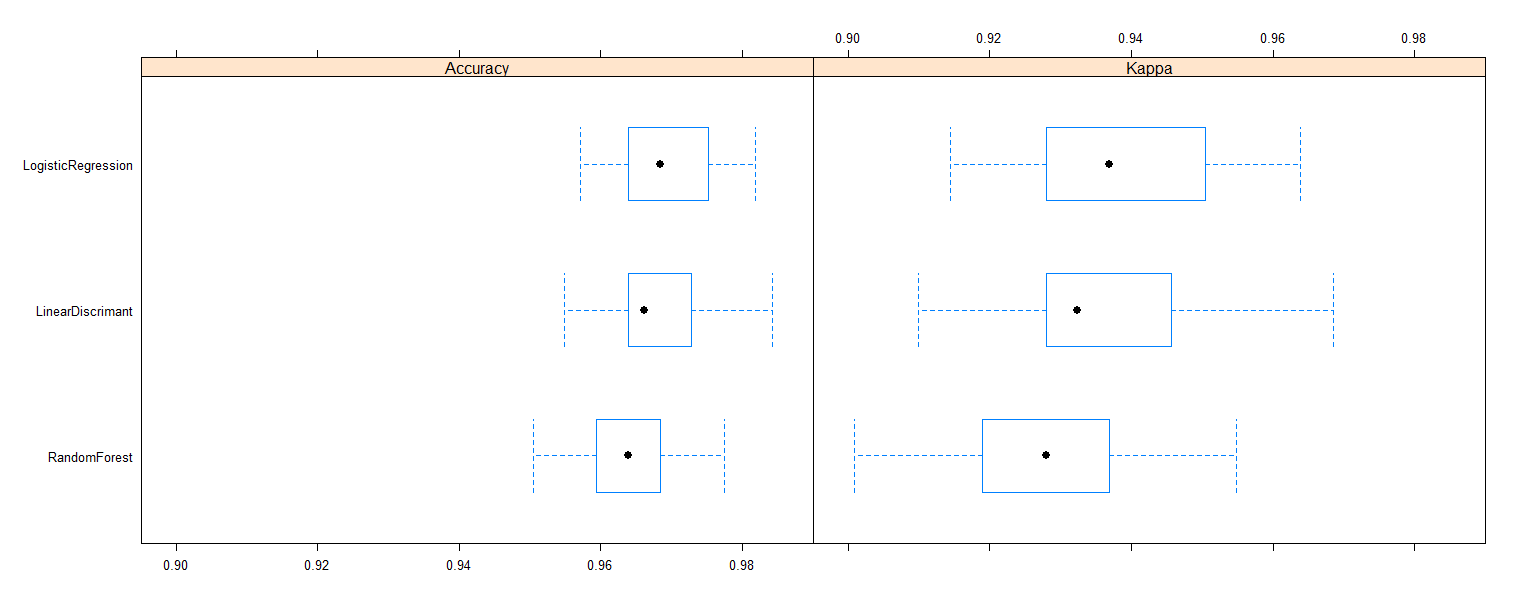
根据结果,我们可以看到,其实逻辑回归的结果还是比较好的。所以我们可以将逻辑回归的结果作为我们最终使用的模型。