电信行业客户流失分析
实验目的
熟悉使用R语言进行大数据综合分析的方法
实验原理
R工具是一套完整的的数据处理计算和制图软件系统。其功能包括:数据存储和处理系统;数组运算工具(其向量、矩阵运算方面功能尤其强大);完整连贯的统计分析工具;优秀的的统计制图功能;简便而强大的的编程语言:可操纵数据的输入和输出以及可实现分支、循环等用户自定义功能。
实验背景
客户在电信运营商中的地位十分重要。在电信业新的市场格局重新确定后,各大电信运营商间的竞争往往首先发生在对客户资源的争夺上。如何有效地挽留住现有客户是电信运营商匝当前日趋激烈的市场竞争中必须重视的环节。然而,电信运营商往往会因为套餐内容或者价格的制定失误导致大量的客户流失。本实验正是想通过数据集中客户对电信运营商服务的使用情况来找出那些导致客户流失的因素,并且做到能够针对某一个客户预测他是否是潜在流失的客户。
实验步骤
- 熟悉R环境;
- 打开R云件环境;
- 在相应编程环境中修改和运行代码;
- 查看结果。
实验一:数据读取
使用提供的电信行业客户流失数据
安装必要的包,如提示包不存在可以用install.packages("包名")的方式安装
library('C50')
library('sjmisc')
library('sjstats')
library('ggplot2')
library('pROC')
train <- read.csv("/data/tele_train_small.csv", header = T)
train_big <- read.csv("/data/tele_train_big.csv", header = T)
test <- read.csv("/data/tele_train_small.csv", header = T)
实验二:数据探索
str(train_big)
'data.frame':    1706496 obs. of  20 variables:
 $ state                        : Factor w/ 51 levels "AK","AL","AR",..: 17 36 32 36 37 2 20 25 19 50 ...
 $ account_length               : int  128 107 137 84 75 118 121 147 117 141 ...
 $ area_code                    : Factor w/ 3 levels "area_code_408",..: 2 2 2 1 2 3 3 2 1 2 ...
 $ international_plan           : Factor w/ 2 levels "no","yes": 1 1 1 2 2 2 1 2 1 2 ...
 $ voice_mail_plan              : Factor w/ 2 levels "no","yes": 2 2 1 1 1 1 2 1 1 2 ...
 $ number_vmail_messages        : num  25 26 0 0 0 0 24 0 0 37 ...
 $ total_day_minutes            : num  265 162 243 299 167 ...
 $ total_day_calls              : int  110 123 114 71 113 98 88 79 97 84 ...
 $ total_day_charge             : num  45.1 27.5 41.4 50.9 28.3 ...
 $ total_eve_minutes            : num  197.4 195.5 121.2 61.9 148.3 ...
 $ total_eve_calls              : num  99 103 110 88 122 101 108 94 80 111 ...
 $ total_eve_charge             : num  16.78 16.62 10.3 5.26 12.61 ...
 $ total_night_minutes          : num  245 254 163 197 187 ...
 $ total_night_calls            : int  91 103 104 89 121 118 118 96 90 97 ...
 $ total_night_charge           : num  11.01 11.45 7.32 8.86 8.41 ...
 $ total_intl_minutes           : num  10 13.7 12.2 6.6 10.1 6.3 7.5 7.1 8.7 11.2 ...
 $ total_intl_calls             : num  5 3 5 7 3 6 7 6 4 5 ...
 $ total_intl_charge            : num  2.7 3.7 3.29 1.78 2.73 1.7 2.03 1.92 2.35 3.02 ...
 $ number_customer_service_calls: int  1 1 0 2 3 0 3 0 1 0 ...
 $ churn                        : Factor w/ 2 levels "yes","no": 2 2 2 2 2 2 2 2 2 2 ...
数据集中包含了19个变量,共1706496行。其中变量洲(state)、国际长途计划(international_plan)、信箱语音计划(voice_mail_plan)和是否流失(churn)为因子变量,其余变量均为数值变量。
实验三:数据预处理
这里的区域编码变量(area_code)没有任何实际意义,故考虑排除该变量。
#剔除无意义的区域编码变量
train <- train[,-3]
train_big <- train_big[,-3]
test <- test[,-3]
#由于模型中,更关心的是流失这个结果(churn=yes),所以对该因子进行排序
train$churn <- factor(train$churn,levels = c('no','yes'), order = TRUE)
train_big$churn <- factor(train_big$churn,levels = c('no','yes'), order = TRUE)
test$churn <- factor(test$churn, ,levels = c('no','yes'), order = TRUE)
实验四:分析建模
对train_big数据构建逻辑回归模型:
#构建Logistic模型
model <- glm(formula = churn ~ ., data = train_big, family = 'binomial')
summary(model)

Call:
glm(formula = churn ~ ., family = "binomial", data = train)

Deviance Residuals:
    Min       1Q   Median       3Q      Max
-1.9364  -0.4994  -0.3130  -0.1663   3.0951

Coefficients:
                                Estimate Std. Error  z value Pr(>|z|)
(Intercept)                   -9.752e+00  4.311e-02 -226.186  < 2e-16 ***
stateAL                        3.578e-01  3.370e-02   10.616  < 2e-16 ***
stateAR                        9.213e-01  3.324e-02   27.717  < 2e-16 ***
stateAZ                        1.097e-01  3.734e-02    2.938  0.00331 **
stateCA                        1.820e+00  3.460e-02   52.600  < 2e-16 ***
stateCO                        6.682e-01  3.369e-02   19.836  < 2e-16 ***
stateCT                        1.034e+00  3.206e-02   32.259  < 2e-16 ***
stateDC                        6.993e-01  3.573e-02   19.571  < 2e-16 ***
stateDE                        7.526e-01  3.313e-02   22.714  < 2e-16 ***
stateFL                        5.983e-01  3.365e-02   17.779  < 2e-16 ***
stateGA                        6.703e-01  3.441e-02   19.483  < 2e-16 ***
stateHI                       -2.158e-01  3.959e-02   -5.451 5.00e-08 ***
stateIA                        2.115e-01  3.988e-02    5.304 1.13e-07 ***
stateID                        8.743e-01  3.306e-02   26.448  < 2e-16 ***
stateIL                       -2.190e-01  3.684e-02   -5.944 2.78e-09 ***
stateIN                        4.549e-01  3.326e-02   13.677  < 2e-16 ***
stateKS                        1.069e+00  3.225e-02   33.153  < 2e-16 ***
stateKY                        8.000e-01  3.384e-02   23.640  < 2e-16 ***
stateLA                        5.638e-01  3.694e-02   15.261  < 2e-16 ***
stateMA                        1.179e+00  3.285e-02   35.896  < 2e-16 ***
stateMD                        1.157e+00  3.168e-02   36.505  < 2e-16 ***
stateME                        1.336e+00  3.220e-02   41.493  < 2e-16 ***
stateMI                        1.402e+00  3.153e-02   44.469  < 2e-16 ***
stateMN                        1.164e+00  3.163e-02   36.793  < 2e-16 ***
stateMO                        6.040e-01  3.422e-02   17.650  < 2e-16 ***
stateMS                        1.362e+00  3.219e-02   42.322  < 2e-16 ***
stateMT                        1.877e+00  3.168e-02   59.263  < 2e-16 ***
stateNC                        6.006e-01  3.334e-02   18.013  < 2e-16 ***
stateND                        1.485e-01  3.520e-02    4.219 2.45e-05 ***
stateNE                        3.055e-01  3.563e-02    8.574  < 2e-16 ***
stateNH                        1.186e+00  3.396e-02   34.907  < 2e-16 ***
stateNJ                        1.581e+00  3.138e-02   50.381  < 2e-16 ***
stateNM                        4.713e-01  3.478e-02   13.552  < 2e-16 ***
stateNV                        1.257e+00  3.205e-02   39.234  < 2e-16 ***
stateNY                        1.171e+00  3.180e-02   36.814  < 2e-16 ***
stateOH                        6.914e-01  3.298e-02   20.966  < 2e-16 ***
stateOK                        8.778e-01  3.343e-02   26.258  < 2e-16 ***
stateOR                        7.706e-01  3.253e-02   23.689  < 2e-16 ***
statePA                        1.156e+00  3.444e-02   33.565  < 2e-16 ***
stateRI                       -1.087e-01  3.626e-02   -2.998  0.00272 **
stateSC                        1.755e+00  3.259e-02   53.856  < 2e-16 ***
stateSD                        8.236e-01  3.367e-02   24.457  < 2e-16 ***
stateTN                        2.700e-01  3.627e-02    7.444 9.77e-14 ***
stateTX                        1.652e+00  3.129e-02   52.782  < 2e-16 ***
stateUT                        1.050e+00  3.289e-02   31.916  < 2e-16 ***
stateVA                       -4.317e-01  3.638e-02  -11.867  < 2e-16 ***
stateVT                        9.838e-02  3.444e-02    2.857  0.00428 **
stateWA                        1.422e+00  3.199e-02   44.462  < 2e-16 ***
stateWI                        2.955e-01  3.449e-02    8.569  < 2e-16 ***
stateWV                        5.767e-01  3.242e-02   17.789  < 2e-16 ***
stateWY                        2.944e-01  3.336e-02    8.826  < 2e-16 ***
account_length                 1.005e-03  6.334e-05   15.868  < 2e-16 ***
international_planyes          2.188e+00  6.762e-03  323.644  < 2e-16 ***
voice_mail_planyes            -2.130e+00  2.627e-02  -81.089  < 2e-16 ***
number_vmail_messages          3.823e-02  8.242e-04   46.384  < 2e-16 ***
total_day_minutes             -6.552e-02  5.946e-02   -1.102  0.27055
total_day_calls                4.028e-03  1.265e-04   31.856  < 2e-16 ***
total_day_charge               4.625e-01  3.498e-01    1.322  0.18614
total_eve_minutes              9.278e-01  7.503e-02   12.365  < 2e-16 ***
total_eve_calls                9.997e-04  1.277e-04    7.832 4.82e-15 ***
total_eve_charge              -1.082e+01  8.827e-01  -12.261  < 2e-16 ***
total_night_minutes           -2.416e-01  3.992e-02   -6.051 1.44e-09 ***
total_night_calls              1.270e-04  1.293e-04    0.982  0.32593
total_night_charge             5.455e+00  8.871e-01    6.149 7.78e-10 ***
total_intl_minutes            -4.214e+00  2.427e-01  -17.363  < 2e-16 ***
total_intl_calls              -9.101e-02  1.137e-03  -80.016  < 2e-16 ***
total_intl_charge              1.592e+01  8.989e-01   17.707  < 2e-16 ***
number_customer_service_calls  5.358e-01  1.810e-03  296.056  < 2e-16 ***
---
Signif. codes:  0 ‘***’ 0.001 ‘**’ 0.01 ‘*’ 0.05 ‘.’ 0.1 ‘ ’ 1

(Dispersion parameter for binomial family taken to be 1)

    Null deviance: 1412246  on 1706495  degrees of freedom
Residual deviance: 1060480  on 1706428  degrees of freedom
AIC: 1060616

Number of Fisher Scoring iterations: 6
可以发现绝大多数的变量已经显著。因为原始数据集条目过多,为了加速之后的试验训练过程,下面换用train_big数据的子集train进行下面的实验。
对train数据重新构建逻辑回归模型:
#构建Logistic模型
model <- glm(formula = churn ~ ., data = train, family = 'binomial')
summary(model)

Call:
glm(formula = churn ~ ., family = "binomial", data = train)

Deviance Residuals:
    Min       1Q   Median       3Q      Max
-1.9200  -0.4994  -0.3127  -0.1664   3.0363

Coefficients:
                                Estimate Std. Error z value Pr(>|z|)
(Intercept)                   -9.753e+00  9.756e-01  -9.996  < 2e-16 ***
stateAL                        3.593e-01  7.627e-01   0.471 0.637573
stateAR                        9.224e-01  7.521e-01   1.226 0.220040
stateAZ                        1.089e-01  8.450e-01   0.129 0.897463
stateCA                        1.821e+00  7.830e-01   2.326 0.020024 *
stateCO                        6.675e-01  7.622e-01   0.876 0.381144
stateCT                        1.034e+00  7.255e-01   1.426 0.153931
stateDC                        6.979e-01  8.086e-01   0.863 0.388065
stateDE                        7.521e-01  7.497e-01   1.003 0.315755
stateFL                        5.983e-01  7.615e-01   0.786 0.432018
stateGA                        6.685e-01  7.788e-01   0.858 0.390694
stateHI                       -2.133e-01  8.960e-01  -0.238 0.811874
stateIA                        2.115e-01  9.022e-01   0.234 0.814665
stateID                        8.738e-01  7.480e-01   1.168 0.242719
stateIL                       -2.206e-01  8.339e-01  -0.265 0.791350
stateIN                        4.539e-01  7.526e-01   0.603 0.546413
stateKS                        1.069e+00  7.297e-01   1.465 0.142794
stateKY                        8.005e-01  7.658e-01   1.045 0.295850
stateLA                        5.629e-01  8.360e-01   0.673 0.500722
stateMA                        1.179e+00  7.433e-01   1.586 0.112673
stateMD                        1.156e+00  7.169e-01   1.613 0.106744
stateME                        1.335e+00  7.287e-01   1.832 0.066916 .
stateMI                        1.403e+00  7.135e-01   1.966 0.049329 *
stateMN                        1.163e+00  7.157e-01   1.625 0.104083
stateMO                        6.023e-01  7.745e-01   0.778 0.436784
stateMS                        1.362e+00  7.283e-01   1.871 0.061408 .
stateMT                        1.878e+00  7.167e-01   2.620 0.008804 **
stateNC                        5.993e-01  7.546e-01   0.794 0.427099
stateND                        1.479e-01  7.966e-01   0.186 0.852729
stateNE                        3.057e-01  8.061e-01   0.379 0.704570
stateNH                        1.186e+00  7.684e-01   1.543 0.122805
stateNJ                        1.581e+00  7.100e-01   2.227 0.025959 *
stateNM                        4.711e-01  7.870e-01   0.599 0.549388
stateNV                        1.257e+00  7.252e-01   1.733 0.083099 .
stateNY                        1.170e+00  7.195e-01   1.626 0.103851
stateOH                        6.909e-01  7.462e-01   0.926 0.354524
stateOK                        8.780e-01  7.564e-01   1.161 0.245733
stateOR                        7.696e-01  7.361e-01   1.045 0.295799
statePA                        1.156e+00  7.793e-01   1.484 0.137936
stateRI                       -1.080e-01  8.203e-01  -0.132 0.895256
stateSC                        1.754e+00  7.376e-01   2.379 0.017379 *
stateSD                        8.233e-01  7.620e-01   1.080 0.279941
stateTN                        2.687e-01  8.209e-01   0.327 0.743377
stateTX                        1.651e+00  7.080e-01   2.332 0.019675 *
stateUT                        1.050e+00  7.442e-01   1.411 0.158358
stateVA                       -4.304e-01  8.231e-01  -0.523 0.601058
stateVT                        9.606e-02  7.797e-01   0.123 0.901945
stateWA                        1.422e+00  7.239e-01   1.965 0.049461 *
stateWI                        2.965e-01  7.804e-01   0.380 0.703980
stateWV                        5.759e-01  7.337e-01   0.785 0.432454
stateWY                        2.953e-01  7.548e-01   0.391 0.695612
account_length                 1.005e-03  1.433e-03   0.701 0.483141
international_planyes          2.188e+00  1.530e-01  14.302  < 2e-16 ***
voice_mail_planyes            -2.131e+00  5.945e-01  -3.584 0.000339 ***
number_vmail_messages          3.824e-02  1.865e-02   2.050 0.040368 *
total_day_minutes             -3.854e-01  3.379e+00  -0.114 0.909187
total_day_calls                4.028e-03  2.861e-03   1.408 0.159188
total_day_charge               2.344e+00  1.988e+01   0.118 0.906114
total_eve_minutes              9.299e-01  1.698e+00   0.548 0.583939
total_eve_calls                1.001e-03  2.889e-03   0.347 0.728889
total_eve_charge              -1.085e+01  1.998e+01  -0.543 0.587089
total_night_minutes           -2.431e-01  9.035e-01  -0.269 0.787842
total_night_calls              1.233e-04  2.926e-03   0.042 0.966392
total_night_charge             5.490e+00  2.008e+01   0.273 0.784494
total_intl_minutes            -4.210e+00  5.492e+00  -0.767 0.443347
total_intl_calls              -9.109e-02  2.575e-02  -3.537 0.000404 ***
total_intl_charge              1.590e+01  2.034e+01   0.782 0.434347
number_customer_service_calls  5.359e-01  4.095e-02  13.084  < 2e-16 ***
---
Signif. codes:  0 ‘***’ 0.001 ‘**’ 0.01 ‘*’ 0.05 ‘.’ 0.1 ‘ ’ 1

(Dispersion parameter for binomial family taken to be 1)

    Null deviance: 2758.3  on 3332  degrees of freedom
Residual deviance: 2071.2  on 3265  degrees of freedom
AIC: 2207.2

Number of Fisher Scoring iterations: 6
发现这时大多数的变量并不显著,故考虑剔除这些不显著的变量,这里使用逐步回归法进行变量的选择(需要注意的是,Logistic为非线性模型,回归系数是通过极大似然估计方法计算所得)。
#step函数实现逐步回归法
model2 <- step(object = model, trace = 0)
summary(model2)

Call:
glm(formula = churn ~ international_plan + voice_mail_plan +
    number_vmail_messages + total_day_charge + total_eve_minutes +
    total_night_charge + total_intl_calls + total_intl_charge +
    number_customer_service_calls, family = "binomial", data = train)

Deviance Residuals:
    Min       1Q   Median       3Q      Max
-2.1204  -0.5133  -0.3375  -0.1969   3.2421

Coefficients:
                               Estimate Std. Error z value Pr(>|z|)
(Intercept)                   -8.067161   0.515870 -15.638  < 2e-16 ***
international_planyes          2.040338   0.145243  14.048  < 2e-16 ***
voice_mail_planyes            -2.003234   0.572352  -3.500 0.000465 ***
number_vmail_messages          0.035262   0.017964   1.963 0.049654 *
total_day_charge               0.076589   0.006371  12.022  < 2e-16 ***
total_eve_minutes              0.007182   0.001142   6.290 3.17e-10 ***
total_night_charge             0.082547   0.024653   3.348 0.000813 ***
total_intl_calls              -0.092176   0.024988  -3.689 0.000225 ***
total_intl_charge              0.326138   0.075453   4.322 1.54e-05 ***
number_customer_service_calls  0.512256   0.039141  13.087  < 2e-16 ***
---
Signif. codes:  0 ‘***’ 0.001 ‘**’ 0.01 ‘*’ 0.05 ‘.’ 0.1 ‘ ’ 1

(Dispersion parameter for binomial family taken to be 1)

    Null deviance: 2758.3  on 3332  degrees of freedom
Residual deviance: 2161.6  on 3323  degrees of freedom
AIC: 2181.6

Number of Fisher Scoring iterations: 6
从结果中发现,所有变量的P值均小于0.05,通过显著性检验,保留了相对重要的变量。模型各变量通过显著性检验的同时还需确保整个模型是显著的,只有这样才能保证模型是正确的、有意义的,下面对模型进行卡方检验。
#模型的显著性检验
anova(object = model2, test = 'Chisq')

Analysis of Deviance Table

Model: binomial, link: logit

Response: churn

Terms added sequentially (first to last)


                              Df Deviance Resid. Df Resid. Dev  Pr(>Chi)
NULL                                           3332     2758.3
international_plan             1  170.400      3331     2587.9 < 2.2e-16 ***
voice_mail_plan                1   41.868      3330     2546.0 9.765e-11 ***
number_vmail_messages          1    3.638      3329     2542.4 0.0564756 .
total_day_charge               1  135.452      3328     2406.9 < 2.2e-16 ***
total_eve_minutes              1   30.874      3327     2376.1 2.753e-08 ***
total_night_charge             1    8.500      3326     2367.6 0.0035509 **
total_intl_calls               1   12.887      3325     2354.7 0.0003309 ***
total_intl_charge              1   16.210      3324     2338.5 5.668e-05 ***
number_customer_service_calls  1  176.839      3323     2161.6 < 2.2e-16 ***
---
Signif. codes:  0 ‘***’ 0.001 ‘**’ 0.01 ‘*’ 0.05 ‘.’ 0.1 ‘ ’ 1
从上图中可知,随着变量从第一个到最后一个逐个加入模型,模型最终通过显著性检验,说明由上述这些变量组成的模型是有意义的,并且是正确的。
虽然模型的偏回归系数和模型均通过显著性检验,但不代表模型能够非常准确的拟合实际值,这就需要对模型进行拟合优度检验,即通过比较模型的预测值与实际值之间的差异情况来进行检验。
Logistic回归模型的拟合优度检验一般使用偏差卡方检验、皮尔逊卡方检验和HL统计量检验三种方法,其中前两种检验适合模型中只有离散的自变量,而后一种适合模型中包含连续的自变量。拟合优度检验的原假设为“模型的预测值与实际值不存在差异”。
#模型的拟合优度检验
HL_test <- hoslem_gof(x = model)
HL_test

$chisq
[1] 13.81744

$df
[1] 8

$p.value
[1] 0.08664957

attr(,"class")
[1] "hoslem_test" "list"
从模型的拟合优度检验结果可知,该模型无法拒绝拟合优度检验的原假设,即可以认为实际值与模型的预测值之间比较接近,不存在显著差异。
以上各项指标均表示模型对电信行业客户流失数据拟合的比较理想,接下来就用该模型对测试集进行预测,预测一个未知的客户是否可能流失,从而起到流失预警的作用。
#模型对样本外数据(测试集)的预测精度
prob <- predict(object = model2, newdata= test, type = 'response')
pred <- ifelse(prob >= 0.5, 'yes','no')
pred <- factor(pred, levels =c('no','yes'), order = TRUE)
f <- table(test$churn, pred)
f

     pred
        no  yes
  no  1408   35
  yes  182   42
实验五:模型评价与优化
1).模型对非流失客户(no)的预测还是非常准确的(1408/(1408+35)=97.6%);
2).模型对流失客户(yes)的预测不理想(42/(182+42)=18.8%)
3).模型的整体预测准确率为87.0%((1408+42)/(1408+35+182+42)),还算说得过去。
实验六:可视化输出
绘制ROC曲线
#绘制ROC曲线
roc_curve <- roc(test$churn,prob)
names(roc_curve)
x <- 1-roc_curve$specificities
y <- roc_curve$sensitivities
p <- ggplot(data = NULL, mapping = aes(x= x, y = y))
p + geom_line(colour = 'red') +geom_abline(intercept = 0, slope = 1) + annotate('text', x = 0.4, y = 0.5, label =paste('AUC=',round(roc_curve$auc,2))) + labs(x = '1-specificities',y = 'sensitivities', title = 'ROC Curve')
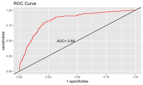
这里的AUC为ROC曲线和y=x直线之间的面积。在实际应用中,多个模型的比较可以通过面积大小来选择更佳的模型,选择标准是AUC越大越好。对于一个模型而言,一般AUC大于0.8就能够说明模型是比较合理的了。